GENSAL

Fifth-order salient-pole synchronous machine. See the shared conventions.

Notes

• \(X''_q=X''_d\) (no subtransient saliency)

• \(X_q=X'_q\)

• \(T'_{q0}\) is neglected

• Only d-axis affected by saturation

Block Diagram

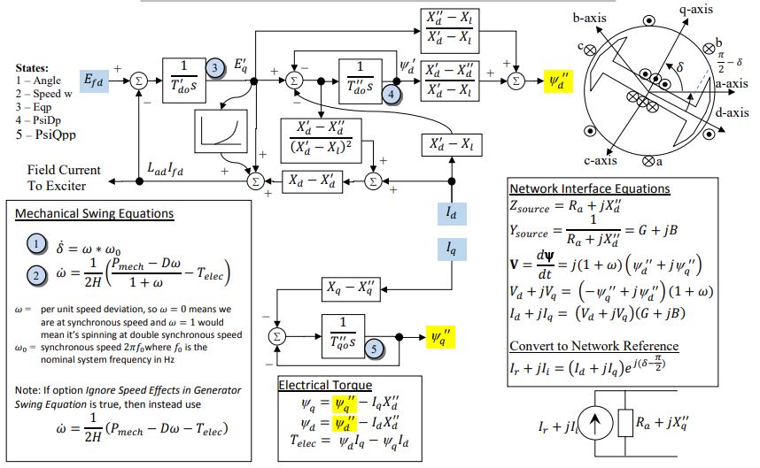
Figure 1: GENSAL. Figure courtesy of PowerWorld

Model Parameters

Symbol	Units	JSON	Description	Typical Value	Note
\(P_0\)	[p.u.]	p0	Initial active power injection	1.0
\(Q_0\)	[p.u.]	q0	Initial reactive power injection	0.0
\(H\)	[s]	H	rotor inertia	3
\(D\)	[p.u.]	D	damping coefficient	0
\(R_\mathrm{a}\)	[p.u.]	Ra	winding resistance	0
\(T'_{d0}\)	[s]	Tdop	Open circuit direct axis transient time const.	7
\(T''_{d0}\)	[s]	Tdopp	Open circuit direct axis sub-transient time const.	0.04
\(T''_{q0}\)	[s]	Tqopp	Open circuit quadrature axis sub-transient time const.	0.05
\(X_d\)	[p.u.]	Xd	Direct axis synchronous reactance	2.1
\(X'_d\)	[p.u.]	Xdp	Direct axis transient reactance	0.2
\(X''_d\)	[p.u.]	Xdpp	Direct axis sub-transient reactance	0.18
\(X_q\)	[p.u.]	Xq	Quadrature axis synchronous reactance	0.5
\(X_{\ell}\)	[p.u.]	Xl	Stator leakage reactance	0.15
\(S_{10}\)	[p.u.]	S10	Saturation factor at 1.0 pu flux	0
\(S_{12}\)	[p.u.]	S12	Saturation factor at 1.2 pu flux	0
\(S^\mathrm{base}\)	[MVA]	mva	Machine power base	100

Parameter Validation

None.

Model Derived Parameters

\[\begin{split}\begin{aligned} G &= \dfrac{R_\mathrm{a}}{R_\mathrm{a}^2+(X''_d)^2} & B &= -\dfrac{X''_d}{R_\mathrm{a}^2+(X''_d)^2}\\ S_A &= \min\left(\dfrac{1.2\sqrt{S_{10}/S_{12}} +1}{\sqrt{S_{10}/S_{12}} +1}, \dfrac{1.2\sqrt{S_{10}/S_{12}} -1}{\sqrt{S_{10}/S_{12}} -1}\right) & S_B &= \dfrac{S_{12}}{(S_A-1.2)^2} \\ X_{d1} &= X_d-X'_d & X_{q2} &= X_q-X''_d \\ X_{d2} &= X'_d-X_\ell & X_{d3} &= (X'_d-X''_d)/X_{d2}^2 \\ X_{d4} &= (X'_d-X''_d)/X_{d2} & X_{d5} &= (X''_d-X_\ell)/X_{d2} \\ f_\mathrm{base} &= f_\mathrm{sys} \end{aligned}\end{split}\]

When \(S_{12}=0\), \(S_A=S_B=0\).

System bases \(f_\mathrm{sys}\) [Hz] and \(S^\mathrm{sys}\) [MVA] are taken from the system at initialization.

Model Ports

Name	Port	Init	Description
bus	Bus	Known	Terminal bus voltage and current-balance residuals
pmech	Input	Unknown	Mechanical-power input; held constant when unconnected
efd	Input	Unknown	Field-voltage input; held constant when unconnected
speed	Output	Known	Machine speed-deviation output

Model Variables

Internal Variables

Differential

Symbol	Units	Description	Note
\(\delta\)	[rad]	Machine internal rotor angle
\(\omega\)	[p.u.]	Machine speed deviation	Optionally read by governor or stabilizer component
\(E'_q\)	[p.u.]	Quadrature axis transient flux
\(\psi'_d\)	[p.u.]	Direct axis transient flux
\(\psi''_q\)	[p.u.]	Total q-axis subtransient flux

Algebraic

Symbol	Units	Description	Note
\(\psi''_d\)	[p.u.]	Total d-axis subtransient flux
\(k_{\mathrm{sat}}\)	[p.u.]	Saturation factor
\(V_d\)	[p.u.]	Machine internal voltage, d-axis
\(V_q\)	[p.u.]	Machine internal voltage, q-axis
\(T_\mathrm{e}\)	[p.u.]	Electrical torque
\(I_d\)	[p.u.]	Terminal current, d-axis
\(I_q\)	[p.u.]	Terminal current, q-axis
\(I_r\)	[p.u.]	Terminal current, real component on network reference frame	Machine base
\(I_i\)	[p.u.]	Terminal current, imaginary component on network reference frame	Machine base

External Variables

Differential

None.

Algebraic

Symbol	Units	Description	Note
\(V_r\)	[p.u.]	Terminal voltage, real component on network reference frame	owned by bus object
\(V_i\)	[p.u.]	Terminal voltage, imaginary component on network reference frame	owned by bus object
\(P_\mathrm{m}\)	[p.u.]	Mechanical power from the prime mover	System base
\(E_{\mathrm{fd}}\)	[p.u.]	Field winding voltage from the excitation system	Machine base

Model Equations

Smooth functions: \(q\).

Internal Equations

Differential

\[\begin{split}\begin{aligned} \dot\delta &= \omega \cdot 2\pi f_\mathrm{base} \\ \dot\omega &= \dfrac{1}{2H}\left(\dfrac{(S^\mathrm{sys}/S^\mathrm{base})P_\mathrm{m}-D\omega}{1+\omega} - T_\mathrm{e}\right)\\ \dot{E}'_q &= \dfrac{1}{T'_{d0}} ( E_{\mathrm{fd}}-E'_q-X_{d1} (I_d+X_{d3}(E'_q-\psi'_d-X_{d2}I_d)) -E'_q k_{\mathrm{sat}} )\\ \dot{\psi}'_d &= \dfrac{1}{T''_{d0}}(E'_q-\psi'_d-X_{d2}I_d)\\ \dot{\psi}''_q &= \dfrac{1}{T''_{q0}}(-\psi''_q-X_{q2}I_q) \end{aligned}\end{split}\]

Algebraic

\[\begin{split}\begin{aligned} 0 &= -\psi''_d + E'_qX_{d5}+\psi'_dX_{d4}\\ 0 &= -k_{\mathrm{sat}} + S_B q(E'_q-S_A)\\ 0 &= -V_d -\psi''_q(1+\omega)\\ 0 &= -V_q +\psi''_d(1+\omega)\\ 0 &= -T_\mathrm{e} +(\psi''_d-I_dX''_d)I_q-(\psi''_q-I_qX''_d)I_d\\ 0 &= -I_d + I_r \sin(\delta) - I_i \cos(\delta) \\ 0 &= -I_q + I_r \cos(\delta) + I_i \sin(\delta) \\ 0 &= -I_r + G (V_d \sin(\delta) + V_q \cos(\delta) - V_r) - B (-V_d \cos(\delta) + V_q \sin(\delta) - V_i) \\ 0 &= -I_i + B (V_d \sin(\delta) + V_q \cos(\delta) - V_r) + G (-V_d \cos(\delta) + V_q \sin(\delta) - V_i) \end{aligned}\end{split}\]

External Equations

The terminal currents are added to the bus residuals on system base:

\[\begin{split}\begin{aligned} I_r^{\mathrm{bus}} &\leftarrow I_r^{\mathrm{bus}} + \dfrac{S^\mathrm{base}}{S^\mathrm{sys}} I_r \\ I_i^{\mathrm{bus}} &\leftarrow I_i^{\mathrm{bus}} + \dfrac{S^\mathrm{base}}{S^\mathrm{sys}} I_i \end{aligned}\end{split}\]

Initialization

Using the power-flow solution, initial currents are calculated from active and reactive power injection. The remaining variables are initialized from the steady-state GENSAL equations.

\[\begin{split}\begin{aligned} \omega &\leftarrow 0 \\ \delta &\leftarrow \text{arg}\left[V_r+jV_i+(R_\mathrm{a}+jX_q)(I_r+jI_i)\right]\\ I_d &\leftarrow I_r\sin(\delta)-I_i\cos(\delta)\\ I_q &\leftarrow I_r\cos(\delta)+I_i\sin(\delta)\\ \psi''_q &\leftarrow -X_{q2}I_q\\ V_d &\leftarrow -\psi''_q\\ V_q &\leftarrow V_r\cos(\delta)+V_i\sin(\delta)+X''_dI_d+R_\mathrm{a}I_q\\ \psi''_d &\leftarrow V_q\\ \psi'_d &\leftarrow \psi''_d-(X''_d-X_\ell)I_d\\ E'_q &\leftarrow \psi'_d+X_{d2}I_d\\ k_{\mathrm{sat}} &\leftarrow S_B q(E'_q-S_A)\\ T_\mathrm{e} &\leftarrow (\psi''_d-I_dX''_d)I_q-(\psi''_q-I_qX''_d)I_d\\ P_\mathrm{m} &\leftarrow \dfrac{S^\mathrm{base}}{S^\mathrm{sys}} T_\mathrm{e}\\ E_{\mathrm{fd}} &\leftarrow E'_q+X_{d1}(I_d+X_{d3}(E'_q-\psi'_d-X_{d2}I_d))+E'_q k_{\mathrm{sat}} \end{aligned}\end{split}\]

Monitors

Monitor	Units	Description	Note
ir	[p.u.]	Terminal current, real component \(\dfrac{S^\mathrm{base}}{S^\mathrm{sys}}I_r\) in the network frame	Oriented leaving the machine; system base
ii	[p.u.]	Terminal current, imaginary component \(\dfrac{S^\mathrm{base}}{S^\mathrm{sys}}I_i\) in the network frame	Oriented leaving the machine; system base
p	[p.u.]	Active power \(P=\dfrac{S^\mathrm{base}}{S^\mathrm{sys}}(V_rI_r+V_iI_i)\)	Oriented leaving the machine; system base
q	[p.u.]	Reactive power \(Q=\dfrac{S^\mathrm{base}}{S^\mathrm{sys}}(V_iI_r-V_rI_i)\)	Oriented leaving the machine; system base
delta	[rad]	Machine internal rotor angle \(\delta\)
omega	[p.u.]	Machine speed deviation \(\omega\)	\(\omega=0\) at synchronous speed
speed	[p.u.]	Per-unit machine speed	\(1+\omega\)
Eqp	[p.u.]	Quadrature-axis transient flux \(E'_q\)	Machine base
psidp	[p.u.]	Direct-axis transient flux \(\psi'_d\)	Machine base
psiqpp	[p.u.]	Total q-axis subtransient flux \(\psi''_q\)	Machine base
psidpp	[p.u.]	Total d-axis subtransient flux \(\psi''_d\)	Machine base
vd	[p.u.]	Machine internal voltage, d-axis \(V_d\)	Machine base
vq	[p.u.]	Machine internal voltage, q-axis \(V_q\)	Machine base
te	[p.u.]	Electrical torque \(T_\mathrm{e}\)	Machine base
id	[p.u.]	Terminal current, d-axis \(I_d\)	Machine base
iq	[p.u.]	Terminal current, q-axis \(I_q\)	Machine base