BranchBreakers

A two-terminal phasor-domain \(\pi\) branch with independently controlled circuit breakers at both terminals.

Notes

• Designed for relay protection: relay trip outputs drive trip1 and trip2, and relays measure the terminal-current outputs.

• Terminal-current outputs publish values without Jacobian coupling to the bus voltages or breaker states.

Block Diagram

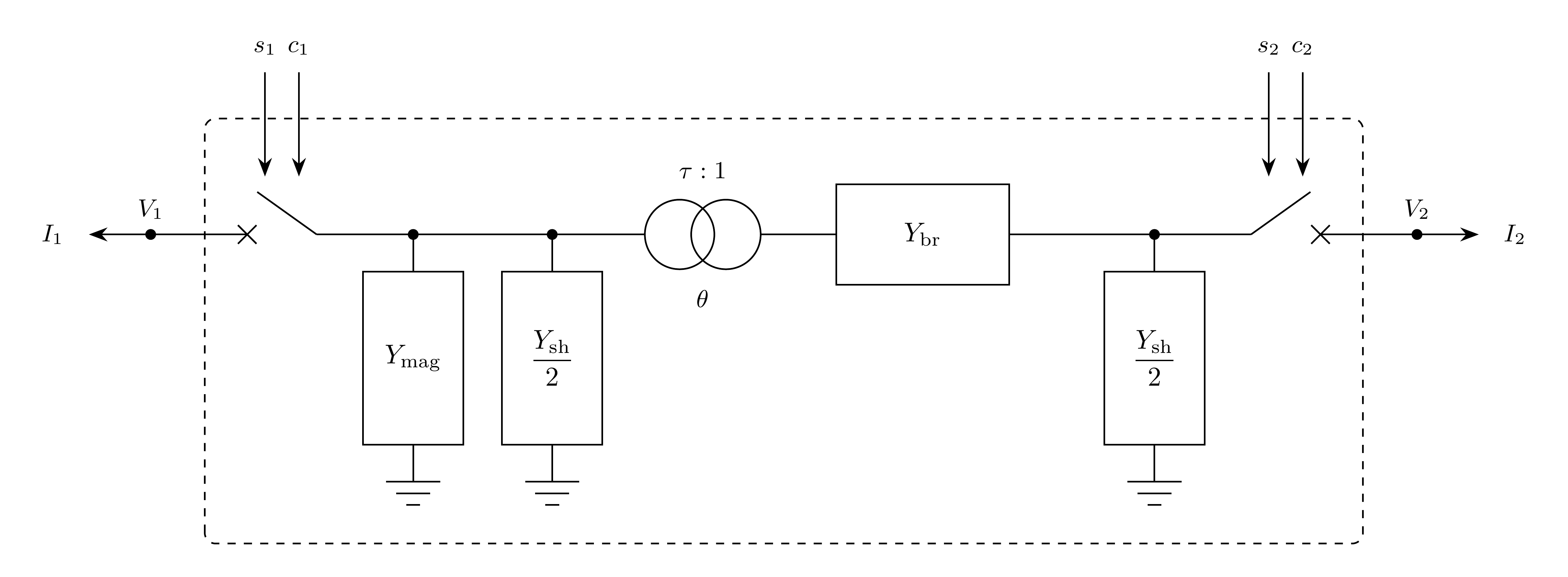
Figure 1: BranchBreakers model.

Model Parameters

Symbol	Units	JSON	Description	Typical Value	Note
\(R\)	[p.u.]	R	Branch series resistance
\(X\)	[p.u.]	X	Branch series reactance
\(G\)	[p.u.]	G	Total line shunt conductance	0.0
\(B\)	[p.u.]	B	Total line shunt susceptance	0.0
\(G_\mathrm{mag}\)	[p.u.]	Gmag	Magnetizing shunt conductance at bus 1	0.0
\(B_\mathrm{mag}\)	[p.u.]	Bmag	Magnetizing shunt susceptance at bus 1	0.0
\(\tau\)	[p.u.]	tap	Off-nominal tap magnitude at bus 1	1.0
\(\theta\)	[rad]	phase	Phase-shift angle	0.0
\(T_\mathrm{brk}\)	[s]	Tbrk	Breaker operating time	0.05	Time to \(z_k = 1/2\) for a unit step command

Parameter Validation

\[\begin{split}\begin{aligned} R^2 + X^2 &> 0 \\ \tau &> 0 \\ T_\mathrm{brk} &\ge 0 \\ Y_{11}, Y_{22} &\ne 0 \end{aligned}\end{split}\]

All parameters must be finite real values.

Model Derived Parameters

\(Y_{mn}\) are entries of the closed-branch admittance matrix \(\mathbf{Y}\). \(Y_k^\mathrm{o}\) is the admittance seen at terminal \(k\) with the opposite breaker open.

\[\begin{split}\begin{aligned} \epsilon_T &= 10^{-3}\ \mathrm{s} \\ T_\mathrm{brk} &\leftarrow \max(T_\mathrm{brk}, \epsilon_T) \\ T_\mathrm{latch} &= \dfrac{T_\mathrm{brk}}{\ln 2} \\ Y_\mathrm{br} &= \dfrac{1}{R + jX} \\ Y_\mathrm{mag} &= G_\mathrm{mag} + jB_\mathrm{mag} \\ Y_\mathrm{sh} &= G + jB \\ \mathbf{Y}_0 &= \begin{bmatrix} -Y_\mathrm{br} & Y_\mathrm{br} \\ Y_\mathrm{br} & -Y_\mathrm{br} \end{bmatrix} \\ \mathbf{Y}_\mathrm{mag} &= \begin{bmatrix} -Y_\mathrm{mag} & 0 \\ 0 & 0 \end{bmatrix} \\ \mathbf{Y}_\mathrm{sh} &= \dfrac{1}{2} \begin{bmatrix} -Y_\mathrm{sh} & 0 \\ 0 & -Y_\mathrm{sh} \end{bmatrix} \\ \mathbf{M} &= \begin{bmatrix} \tau^{-1} & 0 \\ 0 & \exp(j\theta) \end{bmatrix} \\ \mathbf{Y} &= \mathbf{M}^{\dagger}\mathbf{Y}_0\mathbf{M} + \mathbf{Y}_\mathrm{mag} + \mathbf{Y}_\mathrm{sh} \\ Y_1^\mathrm{o} &= Y_{11} - \dfrac{Y_{12}Y_{21}}{Y_{22}} \\ Y_2^\mathrm{o} &= Y_{22} - \dfrac{Y_{21}Y_{12}}{Y_{11}} \end{aligned}\end{split}\]

Model Ports

Name	Port	Init	Description
bus1	Bus	Known	Required bus-1 terminal; the tapped side
bus2	Bus	Known	Required bus-2 terminal
trip1	Input	Known	Bus-1 breaker trip command
close1	Input	Known	Bus-1 breaker close command
trip2	Input	Known	Bus-2 breaker trip command
close2	Input	Known	Bus-2 breaker close command
ir1	Output	Known	Bus-1 terminal current, real component
ii1	Output	Known	Bus-1 terminal current, imaginary component
ir2	Output	Known	Bus-2 terminal current, real component
ii2	Output	Known	Bus-2 terminal current, imaginary component

Signal ports are optional. Attached inputs must be linked. Trip and close commands lie in \([0,1]\); unattached inputs default to zero.

Model Variables

Internal Variables

Differential

Symbol	Units	Description	Note
\(z_1\)	[-]	Bus-1 breaker closed-state latch
\(z_2\)	[-]	Bus-2 breaker closed-state latch

Algebraic

None.

External Variables

Differential

None.

Algebraic

Symbol	Units	Description	Note
\(V_{r1}\)	[p.u.]	Terminal voltage, real component, bus 1	Owned by bus object
\(V_{i1}\)	[p.u.]	Terminal voltage, imaginary component, bus 1	Owned by bus object
\(V_{r2}\)	[p.u.]	Terminal voltage, real component, bus 2	Owned by bus object
\(V_{i2}\)	[p.u.]	Terminal voltage, imaginary component, bus 2	Owned by bus object
\(s_1\)	[-]	Bus-1 breaker trip command	trip1
\(c_1\)	[-]	Bus-1 breaker close command	close1
\(s_2\)	[-]	Bus-2 breaker trip command	trip2
\(c_2\)	[-]	Bus-2 breaker close command	close2

Model Equations

Smooth functions: above, below, latch.

For readability, define:

\[\begin{split}\begin{aligned} u_1 &= \text{above}(z_1; 1/2) \\ u_2 &= \text{above}(z_2; 1/2) \\ \bar{u}_1 &= \text{below}(z_1; 1/2) \\ \bar{u}_2 &= \text{below}(z_2; 1/2) \end{aligned}\end{split}\]

Internal Equations

Differential

\[\begin{split}\begin{aligned} 0 &= -\dot{z}_1 + \dfrac{1}{T_\mathrm{latch}}\text{latch}(z_1, c_1, s_1) \\ 0 &= -\dot{z}_2 + \dfrac{1}{T_\mathrm{latch}}\text{latch}(z_2, c_2, s_2) \end{aligned}\end{split}\]

A close command drives the latch toward closed; a full trip command overrides it.

Algebraic

None.

External Equations

\[\begin{split}\begin{aligned} I_1 &= u_1\left[u_2(Y_{11} V_1 + Y_{12} V_2) + \bar{u}_2 Y_1^\mathrm{o} V_1\right] \\ I_2 &= u_2\left[u_1(Y_{21} V_1 + Y_{22} V_2) + \bar{u}_1 Y_2^\mathrm{o} V_2\right] \end{aligned}\end{split}\]

The real and imaginary parts are added to the bus residuals, positive entering the buses.

Initialization

\[\begin{split}\begin{aligned} z_1 &\leftarrow 1 \\ z_2 &\leftarrow 1 \end{aligned}\end{split}\]

All internal derivatives initialize to zero.

Monitors

Monitor	Units	Description	Note
ir1	[p.u.]	Terminal current, real component, bus 1	\(I_{r1}\)
ii1	[p.u.]	Terminal current, imaginary component, bus 1	\(I_{i1}\)
im1	[p.u.]	Terminal current magnitude, bus 1	\(\sqrt{I_{r1}^2 + I_{i1}^2}\)
p1	[p.u.]	Active power entering bus 1	\(V_{r1} I_{r1} + V_{i1} I_{i1}\)
q1	[p.u.]	Reactive power entering bus 1	\(V_{i1} I_{r1} - V_{r1} I_{i1}\)
ir2	[p.u.]	Terminal current, real component, bus 2	\(I_{r2}\)
ii2	[p.u.]	Terminal current, imaginary component, bus 2	\(I_{i2}\)
im2	[p.u.]	Terminal current magnitude, bus 2	\(\sqrt{I_{r2}^2 + I_{i2}^2}\)
p2	[p.u.]	Active power entering bus 2	\(V_{r2} I_{r2} + V_{i2} I_{i2}\)
q2	[p.u.]	Reactive power entering bus 2	\(V_{i2} I_{r2} - V_{r2} I_{i2}\)