Delay

Delay applies a constant transport delay to each of \(M\) input channels:

\[\mathbf{D}_{\boldsymbol{\tau}}(s) = \mathrm{diag}(\exp(-s\tau_1),\ldots,\exp(-s\tau_M))\]

Block Diagram

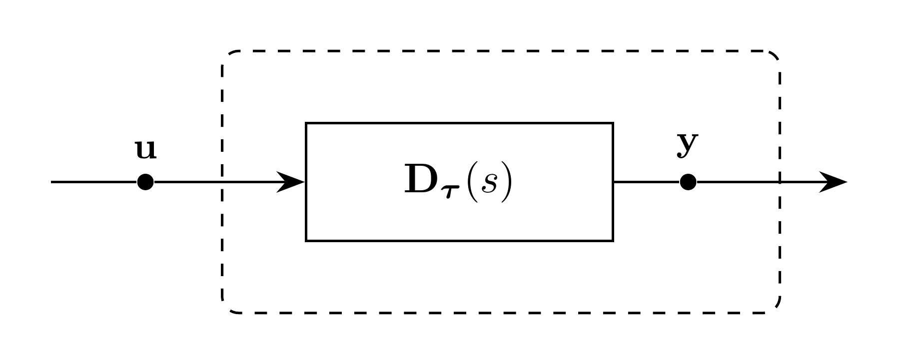
Figure 1: Delay model

Model Parameters

Symbol	Units	JSON	Description	Note
\(M\)	[-]	M	Channel count	Required, positive integer
\(\boldsymbol{\tau}\)	[s]	tau	Channel delays	Required, each positive

Parameter Validation

\[\begin{split}\begin{aligned} M &\in \mathbb{Z}_{>0} \\ \tau_m &> 0 \end{aligned}\end{split}\]

Model Derived Parameters

\[\tau_{\min} = \min(\boldsymbol{\tau}), \qquad \tau_{\max} = \max(\boldsymbol{\tau})\]

Model Ports

Symbol	Port	Type	Units	Description	Note
\(\mathbf{u}\)	input	Input	\([u]\)	Input vector port	\(\mathbf{u} \in \mathbb{R}^M\)
\(\mathbf{y}\)	out	Output	\([u]\)	Delayed output port	\(\mathbf{y} \in \mathbb{R}^M\)

The output provides both value and time derivative.

Submodels

None.

Submodel Validation

None.

Submodel Wiring

None.

Model Variables

History samples are implementation data, not DAE variables or residual rows.

Internal Variables

Differential

None.

Algebraic

None.

External Variables

Differential

None.

Algebraic

Symbol	Units	Description	Note
\(\mathbf{u}\)	\([u]\)	Input vector	\(\mathbf{u} \in \mathbb{R}^M\)

Model Equations

Internal Equations

Differential

None.

Algebraic

None.

External Equations

Each channel satisfies \(y_m(t)=u_m(t-\tau_m)\).

\[\mathbf{y} \leftarrow \mathbf{u}(t-\boldsymbol{\tau})\]

History Realization

History Record

Accepted input history is stored as the knot sequence

\[(t_j,\ \mathbf{u}_j,\ \mathbf{u}'_j), \qquad 0 = t_0 < t_1 < \cdots < t_n\]

where \(\mathbf{u}_j\) and \(\mathbf{u}'_j\) are the input value and derivative at \(t_j\). The first knot holds the initialized values. Channels share knot times and read the record at \(t-\tau_m\) independently.

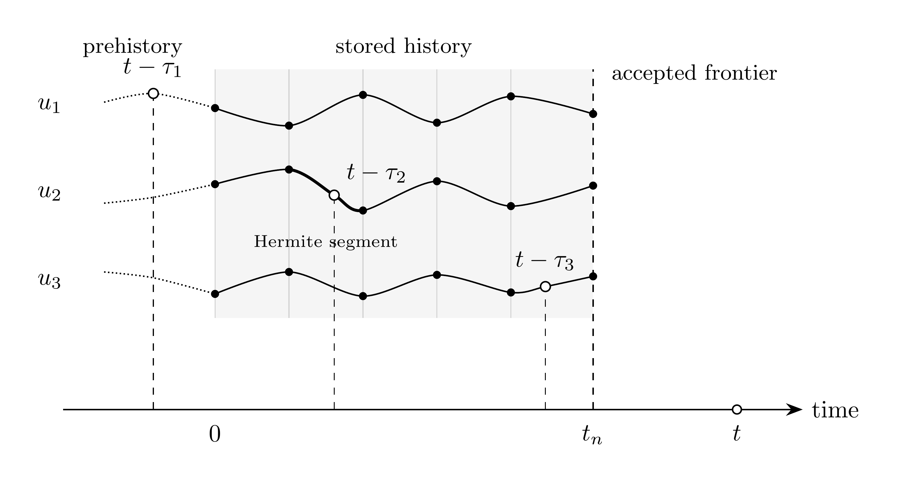
Figure 2: Delay history record and channel taps

Warning

Later knots are appended only at accepted steps, and the solver step size must not exceed \(\tau_{\min}\). These constraints keep every lookup at or behind the accepted frontier; the realization must not extrapolate beyond it.

Interpolation

Suppressing the channel index, a lookup at \(\xi \le 0\) uses the analytic prehistory. For \(\xi \in (t_j,t_{j+1}]\), the bracketing knots define the cubic Hermite interpolant

\[\begin{split}\begin{aligned} h_j &= t_{j+1}-t_j, \qquad \theta = \dfrac{\xi-t_j}{h_j} \\ u(\xi) &= (1-\theta)^2(1+2\theta)\,u_j + \theta(1-\theta)^2\,h_j\,u'_j \\ &\quad + \theta^2(3-2\theta)\,u_{j+1} - \theta^2(1-\theta)\,h_j\,u'_{j+1} \end{aligned}\end{split}\]

Its derivative comes from the same polynomial. For smooth input and exact knot data, the interpolant is \(C^1\) with nominal fourth-order value accuracy and third-order derivative accuracy in the knot spacing.

Initialization

A prehistory for \(\mathbf{u}(t)\) and \(\mathrm{d}\mathbf{u}/\mathrm{d}t\) must be specified over

\[t \in [t_0-\tau_{\max},t_0]\]

Its endpoint value and derivative must match the initialized input at \(t_0\). The delay does not synthesize prehistory. At \(t_0\),

\[\begin{split}\begin{aligned} \mathbf{y} &\leftarrow \mathbf{u}(t_0-\boldsymbol{\tau}) \\ \dfrac{\mathrm{d}\mathbf{y}}{\mathrm{d}t} &\leftarrow \left.\dfrac{\mathrm{d}\mathbf{u}}{\mathrm{d}t} \right|_{t_0-\boldsymbol{\tau}} \end{aligned}\end{split}\]

Monitors

None.